In a previous tutorial, I covered how to predict future stock prices using a deep learning model with 1D CNN layers. This method is effective for basic time series forecasting.
Recently, I've enhanced this model by not just considering past closing prices but also factors like Open, High, Low, Volume, and Adjusted Volume. Furthermore, instead of using 1-D CNN layers, I used transformer encoder to capture contextual information between various stock prices in a time series. This improved the model significantly, cutting the error between the actual and predicted stock prices by more than 50%.
In this tutorial, I will show you how to create a multivariate stock price prediction model using a transformer encoder in TensorFlow Keras. By the end of this article, you'll learn to shape your data for multivariate time series analysis and use a transformer encoder to make a stock price prediction model.
Importing Required Libraries and Datasets
You need to install the following library to access the TensorFlow Keras TransformerEncoder layer.
!pip install keras-nlpSince I used Google Colab to run scripts in this article, I did not have to install any other library. The following script imports the required libraries into our application.
import yfinance as yf
import datetime
import seaborn as sns
import matplotlib.pyplot as plt
from sklearn.model_selection import train_test_split
from sklearn.preprocessing import MinMaxScaler
import numpy as np
import pandas as pd
from datetime import datetime, timedelta
import tensorflow as tf
from keras.models import Model
from keras.layers import Input, Conv1D, MaxPooling1D, Flatten, Dense, Dropout
from keras_nlp.layers import TransformerEncoder
from keras.callbacks import EarlyStopping
from sklearn.metrics import mean_squared_error, mean_absolute_error
Next, we will import the dataset. For the sake of comparison, I will import the same dataset that I used in my previous stock price prediction article. The following script imports the data.
# Define the ticker symbol for the stock
ticker_symbol = "GOOG" # Example: Apple Inc.
# Define the start and end dates for the historical data
# Dataset in the previous article was downloaded on 02-Dec-2023
date_string = "02-Dec-2023"
end_date = datetime.strptime(date_string, "%d-%b-%Y")
start_date = end_date - timedelta(days=5 * 365) # 5 years ago
# Retrieve historical data
data = yf.download(ticker_symbol, start=start_date, end=end_date)
# Display the historical data as a Pandas DataFrame
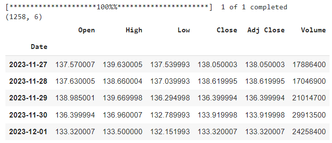
print(data.shape)
data.tail()
Output:
Data Preprocessing for Creating Multivariate Time Series
Before applying the transformer encoder to predict the stock prices, we need to preprocess our dataset and convert it into a shape suitable for training a deep learning model in TensorFlow Keras.
We will divide the dataset into training and test sets and then into corresponding features and label sets. Our feature set will be a multivariate time series.
A multivariate time series is a data point sequence consisting of multiple variables or features. For example, in our case, we have five features (Open, High, Low, Volume, and Adj Close) for a single data point in our sequence. Each feature represents a different aspect of the stock market behavior.
Dividing the Data into Training and Test Sets
The following script divides the data into training and test sets. The training set will be used to train the model, while the test set will be used to evaluate its performance. We will use the last 60 days of data as the test set and the rest as the training set.
We will further divide the training and test sets into corresponding features and labels sets. The feature set will consist of values from the Open, High, Low, Volume, and Adj Close columns of the dataset. The label set will consist of the values from the Close column.
import pandas as pd

# Get the number of records in the DataFrame
total_records = len(data)

# Number of records to keep in the training set
train_size = total_records - 60

# Create the training set
train_data = data.iloc[:train_size]

# Create the test set
test_data = data.iloc[train_size:]

# split each of the training and test sets into features and labels
# Features will include all columns except 'Close'
# Labels will include only the 'Close' column

train_features = train_data.drop('Close', axis=1)
train_labels = train_data['Close']

test_features = test_data.drop('Close', axis=1)
test_labels = test_data['Close']

# Print shapes to confirm
print("Train Features:", train_features.shape, "Train Labels:", train_labels.shape)
print("Test Features:", test_features.shape, "Test Labels:", test_labels.shape)
Output:
Train Features: (1198, 5) Train Labels: (1198,)
Test Features: (60, 5) Test Labels: (60,)
Data Scaling
The next step is to scale the data between 0 and 1. The transformer encoder model works better with normalized data, and the features in our dataset have different scales and units. For example, the Volume feature has much larger values than the Open feature, which can affect the model's performance.
We use the MinMaxScaler from the sklearn library to scale the data. We fit the scaler to the training features and then transform the training and test features with the same scaler. We also reconstruct the dataframes with the original columns and indices for convenience.
We also scale the labels with a separate scaler since we will need to inverse the scaling later to get the actual stock prices.
scaler = MinMaxScaler()

# Fit the scaler to the training features
scaler.fit(train_features)

# Transform the training and test feature sets
train_features_scaled = scaler.transform(train_features)
test_features_scaled = scaler.transform(test_features)

# Reconstruct dataframes with original columns and indices
train_scaled_df = pd.DataFrame(train_features_scaled, columns = train_features.columns, index = train_features.index)
test_scaled_df = pd.DataFrame(test_features_scaled, columns = test_features.columns, index = test_features.index)

scaler = MinMaxScaler()

# Fit the scaler to the training labels and transform them
train_labels = scaler.fit_transform(train_labels.values.reshape(-1, 1))

# Transform the test labels with the already fitted scaler
test_labels = scaler.transform(test_labels.values.reshape(-1, 1))
Creating Multivariate Training and Test Sequences
In this section, we will create multivariate training and test sequences that can be fed to the transformer encoder-based deep learning model. A multivariate sequence is a subset of consecutive data points that consists of multiple features or variables.
To create multivariate sequences, we will use a sliding window approach. We will use a fixed length of data as the input (X) and the next data point as the output (y). For example, if we use a sequence length of 60, we will use the past 60 days of data (Open, High, Low, Volume, and Adj Close) as the input and the next day's closing price as the output. This way, we can capture the temporal dependency of the data and train the model to predict the future price based on past prices.
To create the training set, we will define the create_train_sequence function that takes the normalized training features dataframe, the training labels, and the sequence length as inputs and returns two arrays: X and `y'.
X is an array of multivariate sequences, each with a length of 60 (sequence length), whereas `y' is an array of the next day's closing prices for each sequence. The function will iterate through the dataframe and create sequences by slicing the data.
I used a sequence length of 60 for a fair comparison with the 1D-CNN approach I explained in a previous article.
sequence_length = 60

def create_train_sequence(train_df, train_labels, sequence_length):
    seq_length = sequence_length  # Length of the sequence
    features = []  # List to hold feature sequences
    labels = []    # List to hold labels

    # Iterate through the DataFrame to create sequences
    for i in range(seq_length, len(train_df)):
        sequence = train_df.iloc[i-seq_length:i]  # Get 60 days sequence
        label = train_labels[i]                      # Get the label for the corresponding day

        features.append(sequence.values)  # Append sequence to features
        labels.append(label)              # Append label

    # Convert lists to numpy arrays
    X = np.array(features)
    y = np.array(labels).reshape(-1, 1)

    return X, y
The following script creates the final training features and corresponding labels. You can see the features and labels' shape in the output.
X_train, y_train = create_train_sequence(train_scaled_df,
                                         train_labels,
                                         sequence_length)

print(X_train.shape)
print(y_train.shape)
Output:
(1138, 60, 5)
(1138, 1)
Next, we define the create_test_sequence function that prepares features and labels for the test set. The function takes the normalized training and test dataframes, test labels, and sequence length as parameters.
The create_test_sequence also returns two numpy arrays: X_test and y_test, containing the test features and labels, respectively.
The create_test_sequence function uses a different approach than creating training sequences to create the sequences for the test data, as we want to use the most recent data from the training set and all the data from the test set to make the predictions. The function concatenates the last part of the training data with the test data and then slices the array to get the sequences.
For example, the first record in the test set will have the last 60 days of the training data as the input and the first day of the test data as the output. The second sequence will have the last (60 - 1) days of the training data and the first day of the test data as the input; and the second day of the test data as the output, and so on.
Here is the code for the function create_test_sequence function.
def create_test_sequence(train_df, test_df, test_labels, seq_length):
    # Concatenate the last part of train features with test features
    combined_features_df = pd.concat([train_df.iloc[-seq_length:], test_df])

    test_features = []  # List to hold test feature sequences
    test_labels_list = []  # List to hold test labels

    # Create sequences for the test set
    for i in range(seq_length, len(combined_features_df)):
        sequence = combined_features_df.iloc[i-seq_length:i]  # Get 60 days sequence
        # Use test_labels for label (assuming test_labels is aligned with test_features_df)
        label = test_labels[i - seq_length] if i < len(test_df) + seq_length else None

        test_features.append(sequence.values)  # Append sequence to test features
        test_labels_list.append(label)         # Append label

    # Remove the None values at the end (if any)
    test_features = [feature for feature, label in zip(test_features, test_labels_list) if label is not None]
    test_labels_list = [label for label in test_labels_list if label is not None]

    # Convert lists to numpy arrays
    X = np.array(test_features)
    y = np.array(test_labels_list).reshape(-1, 1)

    return X, y

X_test, y_test = create_test_sequence(train_scaled_df,
                                      test_scaled_df,
                                      test_labels,
                                      sequence_length)
print(X_test.shape)
print(y_test.shape)
Output:
(60, 60, 5)
(60, 1)
Training a Stock Price Prediction Model with Transformer Encoder
We are ready to define our deep learning model containing the Transformer Encoder layer. The model architecture will be similar to the one I created in the 1D CNN article. The only difference will be that, I will replace the CNN layers with TransformerEncoder layer, as shown in the following script.
# input shape: (60 time steps, 5 features)
input_layer = Input(shape=(60, 5))
# Transformer Encoder layers
transformer_1 = TransformerEncoder(num_heads=2, intermediate_dim=64)(input_layer)
dropout_1 = Dropout(0.2)(transformer_1)
transformer_2 = TransformerEncoder(num_heads=2, intermediate_dim=64)(dropout_1)
dropout_2 = Dropout(0.2)(transformer_2)
transformer_3 = TransformerEncoder( num_heads=2, intermediate_dim=64)(dropout_2)
dropout_3 = Dropout(0.2)(transformer_3)
# Flatten layer
flatten = Flatten()(dropout_3)
# Dense layers
dense_1 = Dense(200, activation='relu')(flatten)
# Dense layer
dense_2 = Dense(100, activation='relu')(dense_1)
# Output layer with a single neuron
output_layer = Dense(1, activation='linear')(dense_2)
# Create the model
model = Model(inputs=input_layer, outputs=output_layer)
# Compile the model
model.compile(loss='mean_squared_error', optimizer='adam')
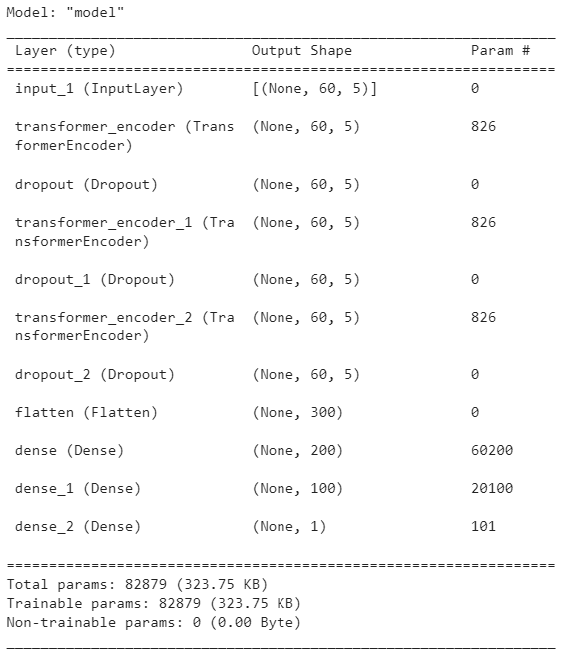
# Display the model summary
model.summary()
Output:
The following script will train the model. Again, this code is similar to the one used for the 1D CNN article.
early_stopping = EarlyStopping(monitor='val_loss', patience=100, restore_best_weights=True)

# Train the model with early stopping
history = model.fit(
    X_train, y_train,
    epochs=500,
    validation_split=0.2,  # 20% of the data for validation
    callbacks=[early_stopping],
    verbose=1
)
Evaluating Model Performance
The following script evaluates the model performance on the test set.
# Make predictions on the test set
predictions = model.predict(X_test)

# Calculate Mean Squared Error (MSE)
mse = mean_squared_error(y_test, predictions)

# Calculate Mean Absolute Error (MAE)
mae = mean_absolute_error(y_test, predictions)

# Print the values
print("Mean Squared Error (MSE):", mse)
print("Mean Absolute Error (MAE):", mae)
Output:
Mean Squared Error (MSE): 0.0025678165444383786
Mean Absolute Error (MAE): 0.0387130112330789
From the above output, we get a mean squared error value of 0.0025, almost 70% less than 0.00839, obtained via the 1D CNN in a previous article.
Similarly, the mean absolute error value of 0.038 is 57% less than 0.0893, obtained via the 1D-CNN.
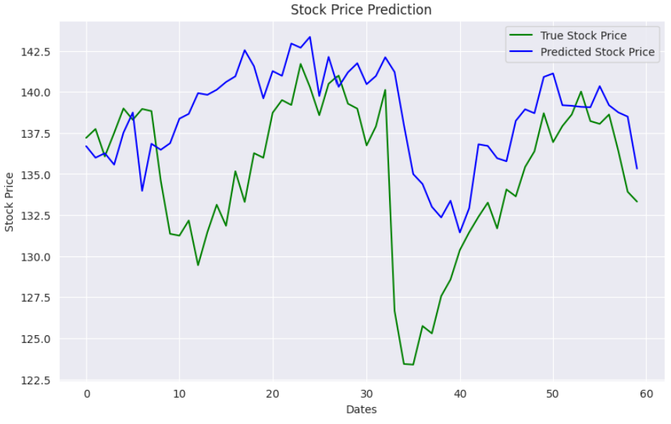
The following script plots the actual and predicted stock values.
# converting predictions and targets to actual values

y_test = scaler.inverse_transform(y_test)
y_true = scaler.inverse_transform(predictions)

plt.figure(figsize=(10,6))
plt.plot(y_test, color='green', label='True Stock Price')
plt.plot(y_true, color='blue', label='Predicted Stock Price')
plt.title('Stock Price Prediction')
plt.xlabel('Dates')
plt.ylabel('Stock Price')
plt.legend()
plt.show()
Output:
Conclusion
In this article, I explained how to create a stock price prediction model in TensorFlow Keras using stacked Transformer encoder layers. The results show that transformer encoder layers significantly outperform the 1D CNN model for stock market price prediction.
I hope you liked the article; feel free to leave feedback or suggestions.