Stock price prediction is a challenging task that requires analyzing historical trends, market sentiments, economic indicators, and company performance. One of the popular methods for stock price prediction is using deep learning models, such as convolutional neural networks (CNNs).
CNNs are a type of neural network that can extract features from sequential and spatial data, such as images, audio, or time series. CNNs consist of multiple layers of convolutional filters that apply a sliding window operation to capture sequential information in the input data.
In this article, we will use a one-dimensional (1D) CNN to predict the stock price of Google (GOOG) based on its historical closing prices. We will use the Python yfinance library to retrieve the historical data from Yahoo Finance. Next, we will use the TensorFlow Keras library to build and train the 1D CNN model. We will also use the Python Scikit learn library for data preprocessing and evaluation.
Importing Required Libraries and Datasets
First, we must import the required libraries and modules for our project.
We will use the following code to import the libraries and modules:
import yfinance as yf
import datetime
import seaborn as sns
import matplotlib.pyplot as plt
from sklearn.model_selection import train_test_split
from sklearn.preprocessing import MinMaxScaler
import numpy as np

import tensorflow as tf
from tensorflow.keras.models import Model
from tensorflow.keras.layers import Input, Conv1D, MaxPooling1D, Flatten, Dense, Dropout
from tensorflow.keras.callbacks import EarlyStopping
from sklearn.metrics import mean_squared_error, mean_absolute_error
Next, we need to define the ticker symbol for the stock price we want to predict. In this case, we will use “GOOG” for Google. We must also define the start and end dates for the historical data we want to download.
We will download the data for the last five years. To do so, we will use the Python datetime module to get the current date and subtract five years from it to get the start date.
We will then use the Python yfinance library to download the historical data from Yahoo Finance. The yfinance library provides the download() function that takes the ticker symbol, the start date, and the end date as parameters and returns a Pandas DataFrame containing the historical data. The DataFrame has six columns: Open, High, Low, Close, Adj Close, and Volume.
The following script downloads the daily stock prices for Google for the last five years.
# Define the ticker symbol for the stock
ticker_symbol = "GOOG"  # Example: Apple Inc.

# Define the start and end dates for the historical data
end_date = datetime.datetime.now()
start_date = end_date - datetime.timedelta(days=5 * 365)  # 5 years ago

# Retrieve historical data
data = yf.download(ticker_symbol, start=start_date, end=end_date)

# Display the historical data as a Pandas DataFrame
print(data.shape)
data.tail()
Output:
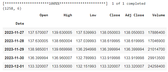
The above output shows that the DataFrame has 1258 rows and six columns, meaning we have 1258 days of historical data for the stock. We can also see the last five rows of the DataFrame, which show the values of the six columns for the most recent days.
To visualize the stock price trend over time, we will use the seaborn and matplotlib libraries to plot the stock's closing price against the date.
plt.figure(figsize=(12, 6))
sns.set_style('darkgrid')
sns.lineplot(x=data.index, y=data['Close'])

# Set plot labels and title
plt.xlabel('Date')
plt.ylabel('Close Price')
plt.title(f'{ticker_symbol} Stock Price Over Time')

# Show the plot
plt.show()
Output:
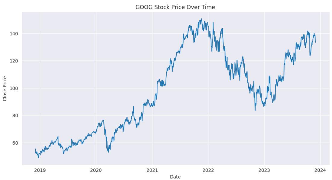
We can see that the stock price has increased significantly over the past five years, with some fluctuations and dips along the way.
Data Preprocessing
Before feeding the data to the 1D CNN model in TensorFlow Keras, we need to perform some data preprocessing steps to make the data suitable for the model.
Firstly, we will divide the data into training and test sets. We will use the last 60 days of data as the test set and the rest as the training set. This way, we can evaluate the model's performance on the most recent data that the model has not seen before.
Note: I tried the past 30 and 60 days of data and got the same results. You can try a different value if you want.
# Divide the dataset into training and test sets

# Get the number of records in the DataFrame
total_records = len(data)

# Number of records to keep in the training set
train_size = total_records - 60

# Create the training set
train_data = data.iloc[:train_size]

# Create the test set
test_data = data.iloc[train_size:]

print(train_data.shape, test_data.shape)
Output:
(1198, 6) (60, 6)
As expected, the training set has 1198 records, and the test set has 60 records.
We will only use the stock's closing price as the input feature for the model. We will also reshape the data from a horizontal array to a vertical array, as required by the MinMaxScaler function that we will use later.
You can try the same experiments on opening, low, high, volume, adjusted closing prices.
train_data = train_data['Close'].values.reshape(-1,1)
test_data = test_data['Close'].values.reshape(-1,1)

print(train_data.shape, test_data.shape)
Output:
(1198, 1) (60, 1)
The above output shows that data has been reshaped from a 2D array to a 1D array, and from a horizontal array to a vertical array.
Next, We will use the MinMaxScaler function from the sklearn library to scale the data to the range of 0 to 1. This will help the model to learn faster and avoid numerical instability issues.
scaler = MinMaxScaler(feature_range = (0, 1))
train_normalized = scaler.fit_transform(train_data)
test_normalized = scaler.transform(test_data)
We will use a sliding window approach to create sequences of data for the model. Each sequence will consist of 60 days of data as the input (X) and the next day’s closing price as the output (y).
For example, the first sequence will have the closing prices from day 1 to day 60 as the input and the closing price from day 61 as the output. The second sequence will have the closing prices from day 2 to day 61 as the input, the closing price from day 62 as the output, and so on.
This way, we can capture the temporal dependency of the data and train the model to predict the future price based on past prices.
The following script defines the create_train_sequences() function that takes the data and the sequence length as parameters and returns two arrays: X and y. X is an array of sequences of data, each with a length of 60. y is an array of the next day’s closing prices for each sequence. The code also defines the sequence length as 60. You can try a different sequence length if you want.
# Create sequences for X_train and y_train
def create_train_sequences(data, sequence_length):
    X, y = [], []
    for i in range(len(data) - sequence_length):
        X.append(data[i:i+sequence_length])
        y.append(data[i+sequence_length])
    return np.array(X), np.array(y)


# Define sequence length
sequence_length = 60
The code below uses the create_train_sequences() function to create X_train and y_train from the normalized training data. The code also prints the X_train and y_train shapes.
X_train, y_train = create_train_sequences(train_normalized , sequence_length)

# Print the shapes of X_train and y_train
print("X_train shape:", X_train.shape)
print("y_train shape:", y_train.shape)
Output:
X_train shape: (1138, 60, 1)
y_train shape: (1138, 1)
We can see that X_train has the shape of (1138, 60, 1), which means that we have 1138 sequences, each with 60 days of data and one feature (the closing price). The label set y_train has the shape of (1138, 1), which means that we have 1138 output values, each corresponding to the next day’s closing price for a sequence.
Next, we will create sequences and labels for the test set. To do so, we will define the create_sequences_test() function, as shown in the following script.
The create_sequences_test() function takes the normalized training and test data as parameters and returns two arrays: X_test and y_test. X_test is an array of data sequences, each with the length of the sequence length parameter, and y_test is an array of the actual closing prices for the test data.
The function uses an approach different than creating training sequences to create the sequences for the test data, as we want to use the most recent data from the training set and all the data from the test set to make the predictions. The function concatenates the last part of the training data with the test data and then slices the array to get the sequences.
For example, the first sequence will have the last 60 days of the training data as the input and the first day of the test data as the output. The second sequence will have the last 59 days of the training data and the first day of the test data as the input; and the second day of the test data as the output, and so on. This way, we can use the most updated information to predict the future price.
# Create X_test and y_test
def create_sequences_test(train_data, test_data):
    X_test, y_test = [], []

    for i in range(len(test_data)):
        X_test.append(np.concatenate((train_data[-(len(test_data) - i):].flatten(), test_data[:i+1].flatten())))
        y_test.append(test_data[i])

    return np.array(X_test)[:, :sequence_length ], np.array(y_test)

# Use the function to create X_test and y_test
X_test, y_test = create_sequences_test(train_normalized, test_normalized)

# Print the corrected shapes of X_test and y_test
print("X_test shape:", X_test.shape)
print("y_test shape:", y_test.shape)
Output:
X_test shape: (60, 60)
y_test shape: (60, 1)
The output shows that X_test has the shape of (60, 60), meaning we have 60 sequences, each with 60 days of data. Similarly, y_test has the shape of (60, 1), which means that we have 60 output values, each corresponding to the actual closing price for a day in the test data.
Training the Models
Now that we have prepared the data, we can build and train the 1D CNN model. The following script defines the model architecture.
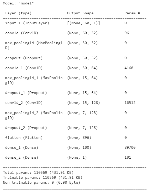
We define an input layer and three convolutional layers, each followed by a max pooling layer and a dropout layer. Next, we define a flatten layer to flatten feature maps received from the final convolutional layer, followed by two dense layers and an output layer.
The code also creates the model object by specifying the input and output layers, compiles the model by specifying the loss function and the optimizer, and displays the model summary, which shows the number of parameters and the output shape of each layer.
# Input layer
input_layer = Input(shape=(sequence_length , 1))

# First Conv1D layer with 32 filters and a kernel size of 3
conv1d_1 = Conv1D(32, 2, activation='relu', padding = 'same')(input_layer)
maxpooling_1 = MaxPooling1D(pool_size=2)(conv1d_1)
dropout_1 = Dropout(0.2)(maxpooling_1)

# Second Conv1D layer with 64 filters and a kernel size of 3
conv1d_2 = Conv1D(64, 2, activation='relu', padding = 'same')(dropout_1)
maxpooling_2 = MaxPooling1D(pool_size=2)(conv1d_2)
dropout_2 = Dropout(0.2)(maxpooling_2)

# Third Conv1D layer with 128 filters and a kernel size of 3
conv1d_3 = Conv1D(128, 2, activation='relu', padding = 'same')(dropout_2)
maxpooling_3 = MaxPooling1D(pool_size=2)(conv1d_3)
dropout_3 = Dropout(0.2)(maxpooling_3)

# Flatten layer
flatten = Flatten()(dropout_3)

# Dense layers
dense_1 = Dense(200, activation='relu')(flatten)

# Dense layers
dense_2 = Dense(100, activation='relu')(flatten)

# Output layer with a single neuron
output_layer = Dense(1, activation='linear')(dense_2)

# Create the model
model = Model(inputs=input_layer, outputs=output_layer)

# Compile the model
model.compile(loss='mean_squared_error', optimizer='adam')

# Display the model summary
model.summary()
Output:
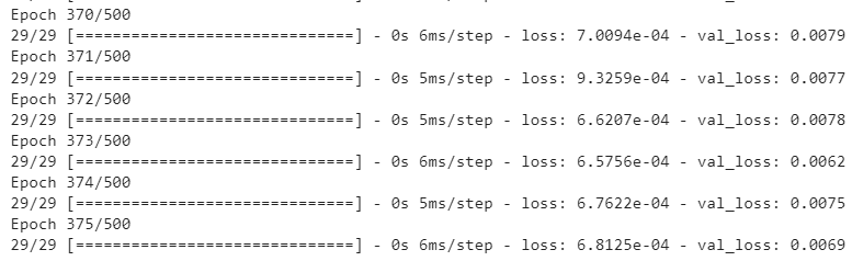
Next, we will train the model for 500 epochs using the fit() method. To evaluate the model during training, we use 20% of training data as the validation set. In addition, we will use the EarlyStopping callback, which monitors the validation loss and stops the training if the validation loss does not improve for a specified number of epochs, which is 100 in our case. The EarlyStopping callback also restores the best weights of the model that achieved the lowest validation loss.
early_stopping = EarlyStopping(monitor='val_loss', patience=100, restore_best_weights=True)

# Train the model with early stopping
history = model.fit(
    X_train, y_train,
    epochs=500,
    validation_split=0.2,  # 20% of the data for validation
    callbacks=[early_stopping],
    verbose=1
)
Output:
Next, we will evaluate the model performance on the test set by making predictions on the test data and calculating the mean squared error (MSE) and the mean absolute error (MAE) between the predictions and the actual values.
## Evaluating the Model Performance on Test Set ##

# Make predictions on the test set
predictions = model.predict(X_test)

# Calculate Mean Squared Error (MSE)
mse = mean_squared_error(y_test, predictions)

# Calculate Mean Absolute Error (MAE)
mae = mean_absolute_error(y_test, predictions)

# Print the values
print("Mean Squared Error (MSE):", mse)
print("Mean Absolute Error (MAE):", mae)
Output:
2/2 [==============================] - 0s 67ms/step
Mean Squared Error (MSE): 0.008394366843826554
Mean Absolute Error (MAE): 0.08936875743648193
The output shows that, on average, our predicted stock price is 8.94% off the actual stock price.
The predictions are made on the scaled test set. We need to convert the scaled values into original stock price values to make a fair comparison. The following script uses the inverse_transform() method to convert the scaled values back to the original values.
# converting predictions and targets to actual values

y_test = scaler.inverse_transform(y_test)
y_true = scaler.inverse_transform(predictions)
Finally, we can plot the actual and predicted stock prices to see how our model performed.
plt.figure(figsize=(10,6))
plt.plot(y_test, color='green', label='True Stock Price')
plt.plot(y_true, color='blue', label='Predicted Stock Price')
plt.title('Stock Price Prediction')
plt.xlabel('Dates')
plt.ylabel('Stock Price')
plt.legend()
plt.show()
Output:
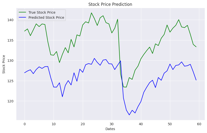
The output shows that our model was able to capture the stock price patterns, though it consistently predicted around 10% less than the actual stock price.
Conclusion
1D convolutional neural networks are a common choice for modeling sequence data. In this article, you saw how to develop a stock price prediction model using a 1D CNN. You can also use the LSTM (long short-term memory network) model for sequence problems. I suggest you try the LSTM model and see how you fare in comparison to CNN. Feel free to comment and share your results and feedback.