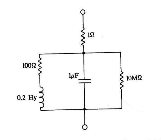
 Here is a version in Python of program from classic Lisp book (see http://www.daniweb.com/software-development/legacy-languages/code/446235/simple-scheme-functions-for-finding-impedance-for-norvigs-implementation for the details) for calculating impedance of a circuit. (Example circuit with 1MOhm like in the book's code not like in diagram)
Calculating impedance of a RLC circuit
from math import pi, degrees
from cmath import phase

def impedance(circuit, omega):
    def r(x):
        return x
    def l(x):
        return complex(0.0, omega * x)
    def c(x):
        return complex(0.0, -1.0 / (omega * x))
    return eval(circuit)

def series(*things):
    return sum(things)

def parallel(*things):
    return 1. / (sum(1. / value for value in things))

if __name__ == '__main__':
    # definition in pairs from LISP implementation
    ##circuit_a = 'series(r(1), parallel(series(r(100.0),l(0.2)), parallel(c(1e-06),r(1000000.0))))'

    # This implementation knows to deal with more than two components in serial/parallel
    circuit_a = 'series(r(1), parallel(series(r(100.0),l(0.2)), c(1e-06),r(1000000.0)))'
    print(circuit_a)

    for omega in 2179.44, 2207.99:
        p = impedance(circuit_a, omega)
        print('omega = %.2f' % omega)
        print(u'rectangular: %.2f + %.2fj' % (p.real, p.imag))
        print(u'polar, angle in degrees: %.2f Ω, φ = %.2f °' % (abs(p), degrees(phase(p))))
print('-'*60) Be a part of the DaniWeb community
We're a friendly, industry-focused community of developers, IT pros, digital marketers, and technology enthusiasts meeting, networking, learning, and sharing knowledge.