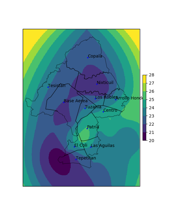
I interpolated temperature data observed on an urban area formed by 12 locations. Now i would like to remove all interpolated values that are outside the shapefile layer. How can i do it?
The shapefile links:
https://www.dropbox.com/s/0u76k3yegvr09sx/LimiteAMG.shp?dl=0
https://www.dropbox.com/s/yxsmm3v2ey3ngsp/LimiteAMG.cpg?dl=0
https://www.dropbox.com/s/yx05n31dfkggbb6/LimiteAMG.dbf?dl=0
https://www.dropbox.com/s/a6nk0xczgjeen2d/LimiteAMG.prj?dl=0
https://www.dropbox.com/s/royw7s51n2f0a6x/LimiteAMG.qpj?dl=0
https://www.dropbox.com/s/7k44dcl1k5891qc/LimiteAMG.shx?dl=0
The Data is:
             Lat       Lon     T
0   20.8208 -103.4434  22.0
1   20.7019 -103.4728  21.9
2   20.6833 -103.3500  24.2
3   20.6280 -103.4261   NaN
4   20.7205 -103.3172  25.7
5   20.7355 -103.3782  24.0
6   20.6593 -103.4136   NaN
7   20.6740 -103.3842  25.0
8   20.7585 -103.3904  23.0
9   20.6230 -103.4265   NaN
10  20.6209 -103.5004  20.0
11  20.6758 -103.6439  26.8
12  20.7084 -103.3901  24.4
13  20.6353 -103.3994  23.1
14  20.5994 -103.4133  23.0
15  20.6302 -103.3422  24.0
16  20.7400 -103.3122  25.3
17  20.6061 -103.3475   NaN
18  20.6400 -103.2900  23.9
19  20.7248 -103.5305  22.2
20  20.6238 -103.2401   NaN
21  20.4400 -103.4200  22.0
22  20.7700 -103.3900  21.0
23  20.7000 -103.4300  25.0
24  20.7100 -103.3700  25.0
25  20.7000 -103.3700  25.0
26  20.6700 -103.3900  23.0
27  20.6700 -103.3200  23.0
28  20.6600 -103.4400  26.0
29  20.6300 -103.4800  23.0
30  20.6200 -103.4800  21.0
31  20.9301 -103.4316  23.0
The code is:
 import cartopy.crs as ccrs
from matplotlib.colors import BoundaryNorm
import matplotlib.pyplot as plt
import numpy as np
import pandas as pd
import cartopy.io.shapereader as shpreader
import matplotlib.pyplot as plt

from metpy.calc import get_wind_components
from metpy.cbook import get_test_data
from metpy.gridding.gridding_functions import interpolate,remove_nan_observations
from metpy.plots import add_metpy_logo
from metpy.units import units

#Definir proyeccion
to_proj = ccrs.AlbersEqualArea(central_longitude=-103.0,central_latitude=20.0)

#Leer datos obervados
data = pd.read_csv('/home/borisvladimir/Documentos/Datos/EMAs/EstacionesZMG/RedZMG.csv', header=0, usecols=(3, 4, 5),names=['Lat', 'Lon', 'T'],na_values=-99999)

#Transforma las coordenadas
lon = data['Lon'].values
lat = data['Lat'].values
xp, yp, _ = to_proj.transform_points(ccrs.Geodetic(), lon, lat).T

#Configura datos nulos
x_masked, y_masked, t = remove_nan_observations(xp, yp, data['T'].values)

#Configura interpolacion radial
tempx, tempy, temp = interpolate(x_masked, y_masked, t, interp_type='rbf', hres=100, rbf_func='linear',rbf_smooth=0.5)
temp = np.ma.masked_where(np.isnan(temp), temp)

#Leer archivo shapefile
fname='/home/borisvladimir/Dropbox/Diversos/Shapes/DistritosZap.shp'
adm1_shapes = list(shpreader.Reader(fname).geometries())

#Configura proyeccion
fig = plt.figure(figsize=(6, 7))
ax = fig.add_subplot(1, 1, 1, projection=to_proj)

#Agrega geometrias del shapefile
ax.add_geometries(adm1_shapes,ccrs.PlateCarree(),edgecolor='black', facecolor='none', alpha=0.5)

#Configura resolucion del mapa
ax.set_extent([-103.60, -103.29, 20.54,20.93 ])

#Agrega etiquetas al mapa
CopaLon,CopaLat=-103.4288,20.8595
TesisLon,TesisLat=-103.5344,20.7857
NixtLon,NixtLat=-103.4043,20.7938
AireLon,AireLat=-103.4922,20.7482
TuzaLon,TuzaLat=-103.4355,20.7333
RobLon,RobLat=-103.4082,20.7576
ArroLon,ArroLat=-103.3540,20.7555
CentroLon,CentroLat=-103.3870,20.7251
VallaLon,VallaLat=-103.4297,20.6834
ColiLon,ColiLat=-103.4634,20.6379
AguiLon,AguiLat=-103.4198,20.6373
TepeLon,TepeLat=-103.4592,20.6062
plt.plot([CopaLon,TesisLon,NixtLon,AireLon,TuzaLon,RobLon,ArroLon,CentroLon,VallaLon,ColiLon,AguiLon,TepeLon],[CopaLat,TesisLat,NixtLat,AireLat,TuzaLat,RobLat,ArroLat,CentroLat,VallaLat,ColiLat,AguiLat,TepeLat],'bo', markersize=2,transform=ccrs.Geodetic())

plt.text(CopaLon-0.0138,CopaLat+0.0098,'Copala',transform=ccrs.Geodetic())
plt.text(TesisLon,TesisLat,'Tesistan',transform=ccrs.Geodetic())
plt.text(NixtLon-0.0138,NixtLat+0.0098,'Nixticuil',transform=ccrs.Geodetic())
plt.text(AireLon-0.0259,AireLat+0.0084,'Base Aerea',transform=ccrs.Geodetic())
plt.text(TuzaLon-0.0138,TuzaLat+0.007,'Tuzania',transform=ccrs.Geodetic())
plt.text(RobLon-0.0359,RobLat+0.005,'Los Robles',transform=ccrs.Geodetic())
plt.text(ArroLon-0.0138,ArroLat+0.007,'Arrollo Hondo',transform=ccrs.Geodetic())
plt.text(CentroLon-0.0138,CentroLat+0.007,'Centro',transform=ccrs.Geodetic())
plt.text(VallaLon-0.0138,VallaLat+0.007,'Patria',transform=ccrs.Geodetic())
plt.text(ColiLon-0.0138,ColiLat+0.007,'El Coli',transform=ccrs.Geodetic())
plt.text(AguiLon-0.0138,AguiLat+0.007,'Las Aguilas',transform=ccrs.Geodetic())
plt.text(TepeLon-0.0138,TepeLat+0.007,'Tepetitan',transform=ccrs.Geodetic())

plt.title('Temperaturas maximas observadas en Zapopan\n8-Feb-2018')
#Configura paleta de colores
levels = list(range(20, 29, 1))
cmap = plt.get_cmap('viridis')
norm = BoundaryNorm(levels, ncolors=cmap.N, clip=True)

mmb = ax.pcolormesh(tempx, tempy, temp, cmap=cmap, norm=norm)
plt.colorbar(mmb, shrink=.4, pad=0.02, boundaries=levels)
plt.show()